A new financial stability risk index to predict the near-term risk of recession
Published as part of the Financial Stability Review May 2018.
The real economy repercussions of financial crises are the ultimate focus of financial stability monitoring and policymakers. By extending a standard set of financial stability indicators with indicators capturing spillover and contagion risks, this special feature proposes a financial stability risk index (FSRI) that has predictive power for the near-term risk of deep recessions. It is shown that the empirical performance of the index benefits from combining a large set of macro-financial indicators and, notably, that the information content of the spillover and contagion risk indicators is important.
1 Introduction
Identifying, measuring and reducing systemic risk is an important part of the task of macroprudential authorities and central banks of safeguarding financial stability. Historical developments have shown that systemic risk can evolve into systemic stress and financial turmoil, with adverse consequences for economic growth and welfare. The large economic cost triggered by the recent global financial crisis is reminiscent of such developments. Therefore, to be able to take appropriate action, policymakers can benefit from an aggregate measure which can adequately capture the potential for instability in the financial system to develop into a large economic downturn.
This special feature builds on recent empirical advances in systemic risk modelling and combines indicators into a composite financial stability risk index (FSRI) to predict near-term large adverse shocks to the real economy. Recent studies suggest that financial condition indicators can provide valuable information about risks to future economic growth, because frictions and fragilities in the financial sector can amplify initial adverse shocks.[1] The magnitude of a financial crisis is thus a result both of the level of imbalances in the economy and the financial sector prior to the crisis and of the extent to which an initial shock is amplified during the crisis. Other studies demonstrate that aggregating various systemic risk indicators can improve the accuracy of forecasting economic activity, in particular in the case of severe recessions.[2] Building on this literature, this special feature presents an FSRI for the euro area that has good near-term predictive power for deep recessions. The index is derived by extracting co-movement information from a large set of indicators covering information both on financial imbalances and on potential amplification risks that may be realised in an ongoing financial turmoil. Combining the information from both types of indicators should enable analysts to make more accurate predictions about adverse economic outcomes. Indeed, tentative results presented in this special feature suggest that the predictive power for near-term risks to GDP growth shocks of this new index is superior to that of individual macro-financial indicators used in financial stability monitoring.
Systemic risk is a multifaceted phenomenon that can be divided into two broad phases.[3] The first phase relates to the build-up of systemic risk, which is characterised by increasing financial imbalances, leverage and exuberance, involving asset price misalignments in the economy. This is often monitored using business and financial cycle measures and their interaction.[4] The second phase relates to the materialisation of systemic risk, i.e. when the transmission of a shock is endogenously amplified by fragilities and frictions within the system. Such amplification and contagion risk is more closely linked to the interconnectedness of financial institutions, whose direct or indirect business relationships may eventually contribute to the level of systemic stress experienced during a crisis. In the monitoring of risks to financial stability, the focus is on assessing the probability that a systemic crisis will materialise, whereas in the monitoring of spillover and contagion risks, the effort is put on assessing the overall damage that a shock could inflict on the financial system.[5] Hence, the risk build-up is usually measured in the time dimension, while shock amplification is seen in terms of the cross-sectional or cross-border dimension (see Figure A.1).
The multifaceted nature of systemic risk justifies a broad-based analytical approach
Topology of systemic risk and the mapping of modelling approaches

Source: ECB.
This special feature focuses on the near-term predictive properties of financial stability indicators. The approach presented here combines information on cyclical systemic risks with information on contagion and spillover risks, not only with a view to anticipating an imminent downturn, i.e. in the next quarter, but also with the aim of assessing how large the downturn could be. For that purpose, it extends a standard set of macro-financial variables on measuring systemic risk[6] with indicators designed to capture contagion and spillover risk. Meanwhile, Special Feature B focusses on cyclical systemic risk and therefore on a longer prediction horizon of two to three years for the likelihood of a financial crisis.
2 Review and taxonomy of existing indicators
A broad-based analytical approach is beneficial for effective monitoring of systemic risk. Asset price misalignments, excessive leverage and maturity mismatches are examples of cyclical vulnerabilities, while a high degree of interconnectedness, e.g. lending and funding relationships involving sizable volumes, and overlapping portfolios could give rise to adverse second-round effects. For cyclical systemic risk monitoring, models based on time series are the most appropriate analytical device. These include early warning models based on credit and financial market indicators. Monitoring of contagion and spillover risks is usually based on network, spillover and contagion models or reduced-form conditional loss probability models. These models make use of cross-sectional information.
The main value of financial stability indicators lies in whether they predict severe recessions caused by amplifications of financial imbalances. The effects of materialising systemic risk concern the left tail of the real economic growth density when an initial shock is endogenously aggravated by the activation of multiple vicious spirals, such as the bank-sovereign nexus, macro-financial negative feedback loops, liquidity spirals and fire sales. Vulnerability indicators that are good predictors of the materialisation of systemic crises are well documented in the literature.[7] However, there has been less research on the extent to which financial stability or systemic risk measures are useful in gauging the magnitude of a crisis.[8]
A comprehensive set of financial stability indicators should cover both cyclical and cross-sectional measures. This special feature uses the taxonomy shown in Figure A.2.[9] It divides the set of macro-financial variables into four buckets, the first three being standard categories of indicators for systemic risk monitoring: (i) valuation pressures and risk appetite, which cover indicators that mostly reflect asset price developments, (ii) non-financial sector imbalances, which are captured mostly by debt developments in that sector, (iii) financial sector risks, which are measured by a set of leverage indicators and concentration measures. The fourth is a new category introduced in this special feature consisting of a set of 16 measures of spillover and contagion risks that may serve as yardsticks for the potential amplification of initial shocks.
Taxonomy of macro-financial indicators for financial stability analysis
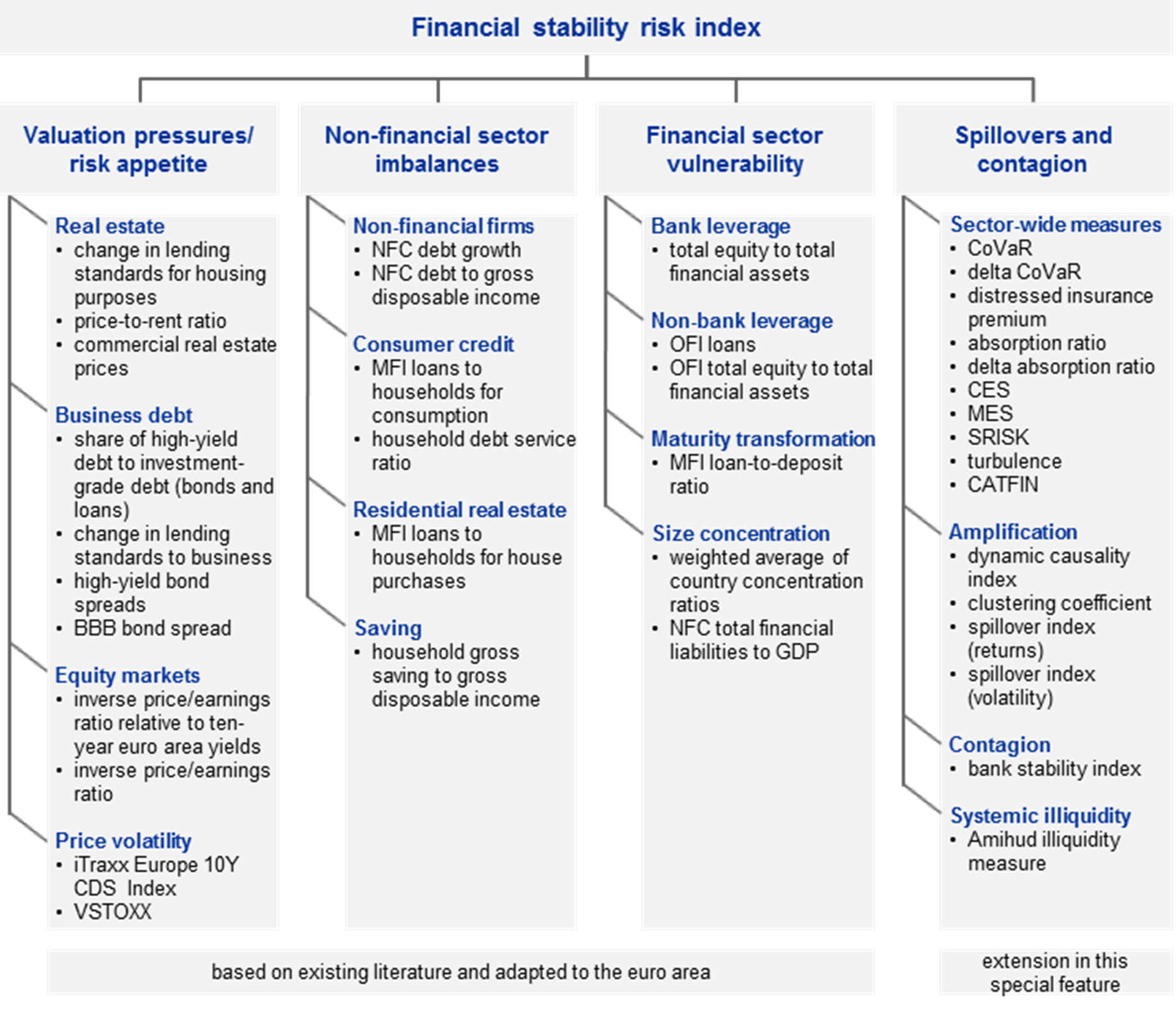
Sources: Aikman et al. (2017) and ECB.Note: See Table A.1 for an explanation of spillover and contagion measures.
The measures of spillovers and contagion could be further classified into four broad sub-categories. Sector-wide measures cover the indicators of overall systemic risk that can also be decomposed into the contributions of individual financial institutions. Interconnectedness or amplification measures are standard network indicators assessing the importance of the nodes or network concentration, such as the degree of the centrality of the networks. Contagion measures are based on simulation of default cascades in the networks, while systemic risk-taking indicators relate to systemic liquidity in the financial system. The indicators and the purpose of their measurement are summarised in Table A.1. Overall, this four bucket approach can also be distilled from the broad literature on systemic risk indicators.[10]
Yardsticks of spillovers and contagion risks could be useful in assessing the potential magnification effect of an initial shock. Measures of spillovers and contagion may contain information about the degree by which risks could be amplified when they materialise. As such, they could be helpful in assessing the cost of crises in terms of the scale of economic downturns.[11]
Measures of cross-sectional systemic risks
Classification and characteristics of cross-sectional systemic risk indicators
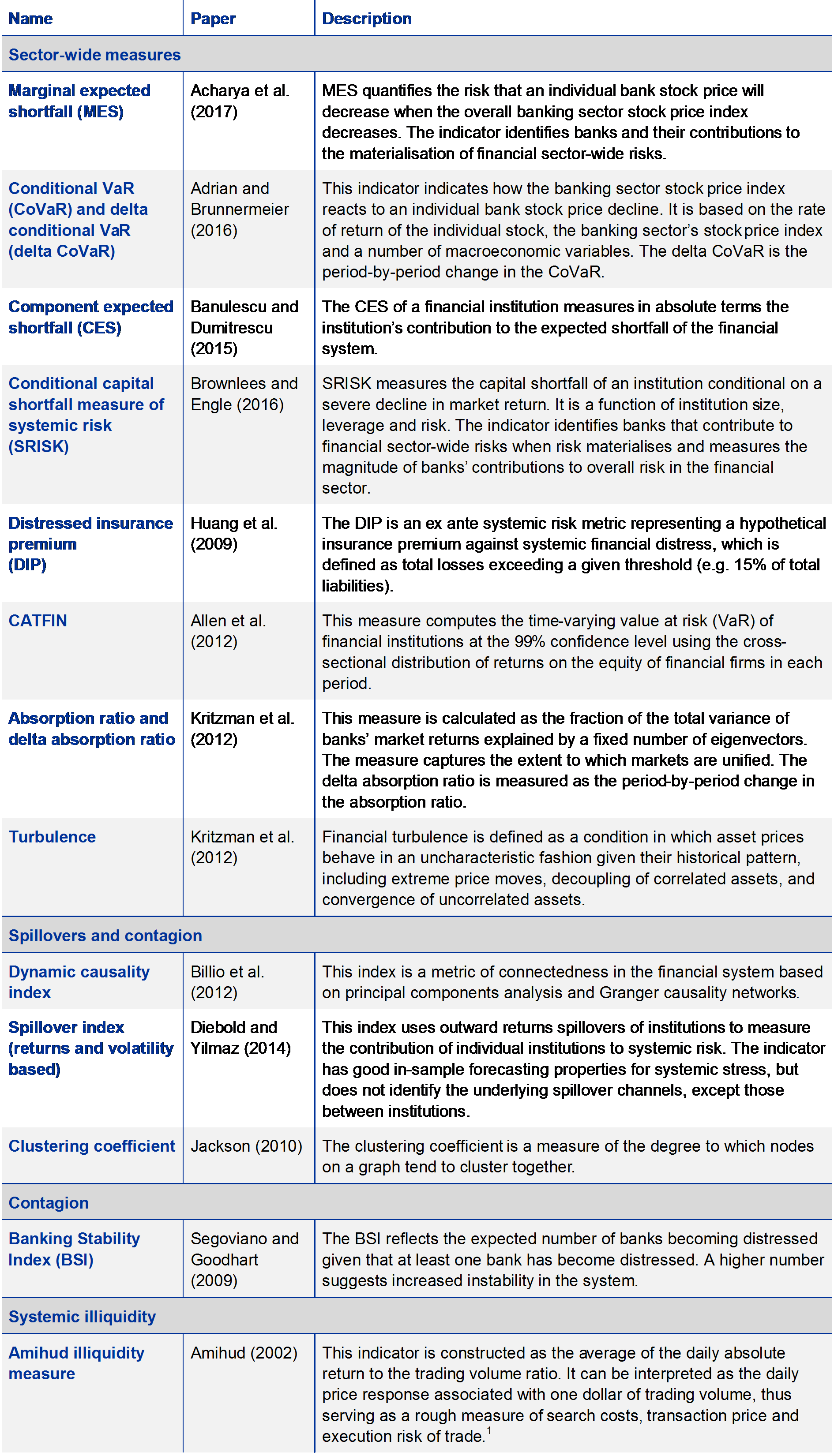
Source: ECB calculations.Notes: Bibliographical references: Acharya, V.V., Pedersen, L.H., Philippon, T. and Richardson, M., “Measuring Systemic Risk”, The Review of Financial Studies, Vol. 30(1), 2017, pp. 2-47.Adrian, T. and Brunnermeier, M.K. “CoVaR”, American Economic Review, Vol. 106(7), 2016, pp. 1705-1741.Allen, L., Bali, T.G. and Tang, Y., “Does Systemic Risk in the Financial Sector Predict Future Economic Downturns?”, The Review of Financial Studies, Vol. 25(10), 2012, pp. 3000-3036.Amihud, Y., “Illiquidity and stock returns: cross-section and time-series effects”, Journal of Financial Markets, Vol. 5(1), 2002, pp. 31-56.Banulescu, G.-D., and Dumitrescu, E.-I., “Which are the SIFIs? A Component Expected Shortfall approach to systemic risk”, Journal of Banking & Finance, Vol. 50, 2015, pp. 575-588.Billio, M., Getmansky, M., Lo, A.W. and Pelizzon, L., “Econometric measures of connectedness and systemic risk in the finance and insurance sectors”, Journal of Financial Economics, Vol. 104(3), 2012, pp. 535-559.Brownlees, C. and Engle, R.F., “SRISK: A Conditional Capital Shortfall Measure of Systemic Risk”, The Review of Financial Studies, Vol. 30(1), 2017, pp. 48-79.Diebold, F.X. and Yılmaz, K., “On the network topology of variance decompositions: Measuring the connectedness of financial firms”, Journal of Econometrics, Vol. 182(1), 2014, pp. 119-134.Huang, X., Zhou, H. and Zhu, H., “Systemic Risk Contributions”, Journal of Financial Services Research, Vol. 42(1-2), 2012, pp. 55-83.Jackson, M.O., Social and Economic Networks, Princeton University Press, 2010.Kinlaw, W., Kritzman, M. and Turkington, D., “Toward Determining Systemic Importance”, The Journal of Portfolio Management, Vol. 38(4), 2012, pp. 100-111.Segoviano, M.A. and Goodhart, C.A.E., “Banking Stability Measures”, IMF Working Paper, No 09/4, International Monetary Fund, 2009.1) Surges in search costs, transaction prices and execution risks of trades are signs of market liquidity vaporising in times of turmoil, as evidenced in the recent financial crisis (see, for example, Gârleanu, N. and Pedersen, L.H., “Liquidity and Risk Management”, American Economic Review, Vol. 97(2), 2007, pp. 193-197; and Brunnermeier, M.K. and Pedersen, L.H., “Market Liquidity and Funding Liquidity”, The Review of Financial Studies, Vol. 22(6), 2009, pp. 2201-2238). These stem from heightened information and agency frictions, such as adverse selection, spreading through an interconnected financial system. Amihud market illiquidity captures such contagion of uncertainty and information frictions in interconnected markets (see Amihud, Y., op. cit.).
Box AConstruction and estimation of a financial stability risk index by means of partial quantile regression
This box describes in more detail the specific methodology used to construct the FSRI. The analysis is split into two main steps: (i) condensing relevant information contained in the broad set of indicators and systemic risk measures into a small number of components, and (ii) evaluating the predictive power of these components for large economic downturns.
The large set of variables and indicators is aggregated into a small number of factors that capture the salient features of the underlying data. Specifically, for each of the four classes of indicators in the taxonomy shown in Figure A.2, one factor is extracted. At the technical level, reducing the data dimension has the objective of retrieving information from the underlying indicators which may otherwise be obscured by measurement error. This allows a robust predictive relationship with real economic developments, notably large downturns, to be established. In addition, relative to including a large set of indicators in regression analysis, the extracted common signal should mitigate in-sample overfitting problems.
The forecast target for real economic outcomes is shocks to quarterly real GDP growth one quarter ahead. The purpose of this special feature is not to predict the level of GDP growth, as the systemic risk indicators and the macro-financial indicators are unlikely to contain sufficient information for that purpose. However, if these variables are useful for systemic risk analysis, they should be informative for large unexpected shocks to GDP growth. An empirical measure of such shocks can be approximated by the residuals from an autoregressive process for quarter-on-quarter real GDP growth.[12] This strips out variation that can be predicted from past realisations of GDP alone and preserves the purely unexpected portion to be forecast by the FSRI. In the next step, a quantile regression is carried out in which the factor summarising the systemic risk and macro-financial variables is used to predict the left tail of the GDP growth density.
For the predictor, information from the comprehensive set of indicators is aggregated into the FSRI using partial quantile regression. This dimension reduction prevents data-overfitting issues caused by having a large number of indicators as predictors. It extends the concept of partial least squares to quantile regression and proceeds in two stages. The common component or factor across variables is computed in the first stage. In the second stage, the GDP disturbances one period ahead are regressed on the factor from the first stage. In the first stage, the quantile-specific slope coefficients of each explanatory variable with respect to the GDP shocks are found through quantile regressions.[13] The factor estimate at each point in time is then computed from a recursive regression of the explanatory variables on the slope coefficients. Effectively, this implies that the factor is computed as the cross-sectional covariance estimate of the explanatory variables with the slope estimates. In the second stage, the factor serves as the explanatory variable in the predictive quantile regression of the GDP shocks.[14] The construction of factors and the predictive regression are carried out recursively over time in order to avoid the inclusion of future information in parameter estimates.[15]
The forecast performance is evaluated by a goodness-of-fit measure akin to in linear regression but amended for the quantile set-up. Specifically, the quantile used here is defined as
where the numerator of the fraction captures the loss from the quantile regression computed from the estimated residuals and is the quantile loss function with respect to the quantile .[16] The denominator captures the unconditional quantile estimate, i.e. the loss associated with the difference between GDP shocks and their -th quantile. That is, in this setting the statistical significance of the out-of-sample estimates is assessed by comparing the conditioning information (the numerator) with the unconditional historical quantile (the denominator).
As a robustness check, two alternative data reduction methods for the first stage of the analysis were tested and they led to similar results to the partial quantile regression approach. The first alternative approach uses principal component analysis to extract a common component from the macro-financial indicators. The principal component methodology condenses the information in the macro-financial indicators according the covariance among them.[17] The second approach is based on a dynamic factor model with time-varying parameters.[18] This methodology extends the principal component analysis to allow for autocorrelation in the factor and assumes a priori that parameters are time-varying, as opposed to the recursive estimations where the a priori assumption is that the parameters of the model are constant. The detailed results of these alternative ways of computing the factor in the first stage are not reported in this special feature, but the results are qualitatively similar to those obtained from the partial quantile regression approach. However, the results of the latter are superior to those of the two alternative approaches according to the goodness-of-fit criteria.
3 A financial stability risk index for the euro area
The proposed FSRI for the euro area incorporates relevant information extracted from the large set of indicators of cyclical and cross-sectional vulnerabilities. Specifically, data dimension reduction is applied to efficiently aggregate information across indicators, which is useful for predicting large economic downturns. Box A explains the methodology for the construction of the index and the methodology for the assessment of its performance in predicting large economic downturns in greater detail. The reminder of this section presents the new index and its empirical properties (see Chart A.1).
The FSRI rises just before large economic downturns
FSRI and large recessions
(index; Q1 2000 – Q4 2017)
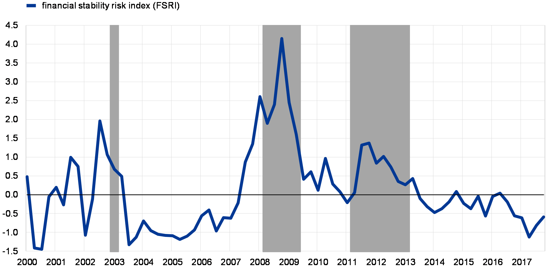
Sources: ECB and ECB calculations.Notes: The grey-shaded areas show periods in which quarterly GDP growth was below the 20th percentile of the historical distribution of GDP growth rates from 1995 to 2017. At each point in time the index is standardised by its historical mean and standard deviation. The standardisation of the first 12 quarters is for that period.
The proposed FSRI provides a comprehensive view on the level of near-term financial stability risks with negative repercussions for the real economy. The level of the index suggests that systemic risk in the euro area has decreased since the sovereign debt crisis in 2011/12 and that it has been below its long-term average since the second half of 2013. Nevertheless, the average level of the index observed in that period exceeded levels observed in the period between the middle of 2003 and the end of 2006. This is in contrast to the readings from other financial stability indicators based mostly on market prices, which, owing to currently depressed risk premiums, signal a low level of risk. Because it also includes non-price-based indicators, the new index is less susceptible to the volatility paradox, whereby crises are often preceded by periods of very low volatility in financial markets.
The FSRI captures well the most important events during the recent crisis episodes. It increases at the outbreak of the sub-prime crisis in the third quarter of 2007 and reaches a first peak in the first quarter of 2008 when Bear Stearns was bailed out. Indeed, following this peak quarterly real GDP growth turned negative to ‑0.4% in the second quarter of 2008, reaching the 20th percentile of the historical growth distribution. The index reaches an all-time high in the fourth quarter of 2008, when the global economy began collapsing after the default of Lehmann Brothers in September 2008. Afterwards, quarterly GDP growth fell to its lowest observed value of -2.9% in the first quarter of 2009. The index increased again at the height of the euro area sovereign debt crisis in 2011 and 2012, when market analysts speculated about redenomination risk in the euro area. Quarterly GDP growth rates were negative between the fourth quarter of 2011 and the first quarter of 2013, since when the index has been gradually receding (see Chart A.1).
The index provides accurate short-term predictions of large economic downturns. While the build-up of vulnerabilities may take time, the precise timing of the eruption of a systemic crisis is hard to pinpoint, as the initial triggers of such events are unpredictable. Nevertheless, spillovers and contagion effects may shed light on the extent of possible amplification once the negative shock materialises. The FSRI seems to perform well in predicting large negative readings of GDP growth by providing accurate short-term forecasts of negative shocks to GDP growth (see Chart A.2).
The FSRI provides accurate near-term predictions of deep recessions …
One-quarter out-of-sample forecasts of shocks to euro area real GDP growth
(Q1 2005 to Q4 2017; quarterly percentage changes)

Sources: ECB and ECB calculations.Note: The one-quarter-ahead out-of-sample forecast is aligned with the realised quarterly shock.
The sensitivity of the index increases around episodes of large economic downturns. Since the indicators of spillovers and contagion provide information about the potential for the amplification of the initial shock, their information content could be particularly relevant during episodes of systemic stress. This is mirrored by more negative regression coefficients of the quantile factors, which point to higher sensitivity of the indicator in explaining GDP growth shocks. These coefficients reached significantly more negative values in 2008 and remained low during the periods of the global financial crisis and the euro area sovereign debt crisis before recovering again in 2012 (see Chart A.3).
… and its sensitivity increases around systemic crises
Recursive quantile regression coefficients of one-quarter out-of-sample forecasts
(Q1 2005 to Q4 2017; coefficient values)

Sources: ECB and ECB calculations.Note: Quantile process coefficients multiplying the factor in recursive quantile regressions starting in the first quarter of 2005.
Large economic downturns are better predicted by aggregating information embedded in individual indicators. Combining efficiently all individual indicators together into a synthetic measure of financial stability improves its predictive power compared to the aggregation of individual risk indicators. The index outperforms the forecasting power of individual indicators and their subsets. Sub-indices derived for the four risk categories according to the proposed taxonomy (see Figure A.2) and using the same aggregation method perform worse than the overall index in predicting shocks to real GDP growth (see Chart A.4).
Indicators of spillover and contagion do have predictive power, in particular for large economic downturns. Among the sub-indices, cross-sectional systemic risk valuation pressure indicators tend to contain the most information for explaining large economic declines as measured by the 25th percentile of shocks to GDP growth. Notably, a sub-index constructed from all cyclical indicators and the spillover and contagion risk sub-index perform similarly well in predicting large economic downturns. However, both sub-indices are outperformed by the overall index (see Chart A.4).
Aggregating individual indicators into an FSRI improves overall predictive power …
One quarter out-of-sample forecast accuracy of the index and its sub-indices
(normalised predictive accuracy; percentage points)
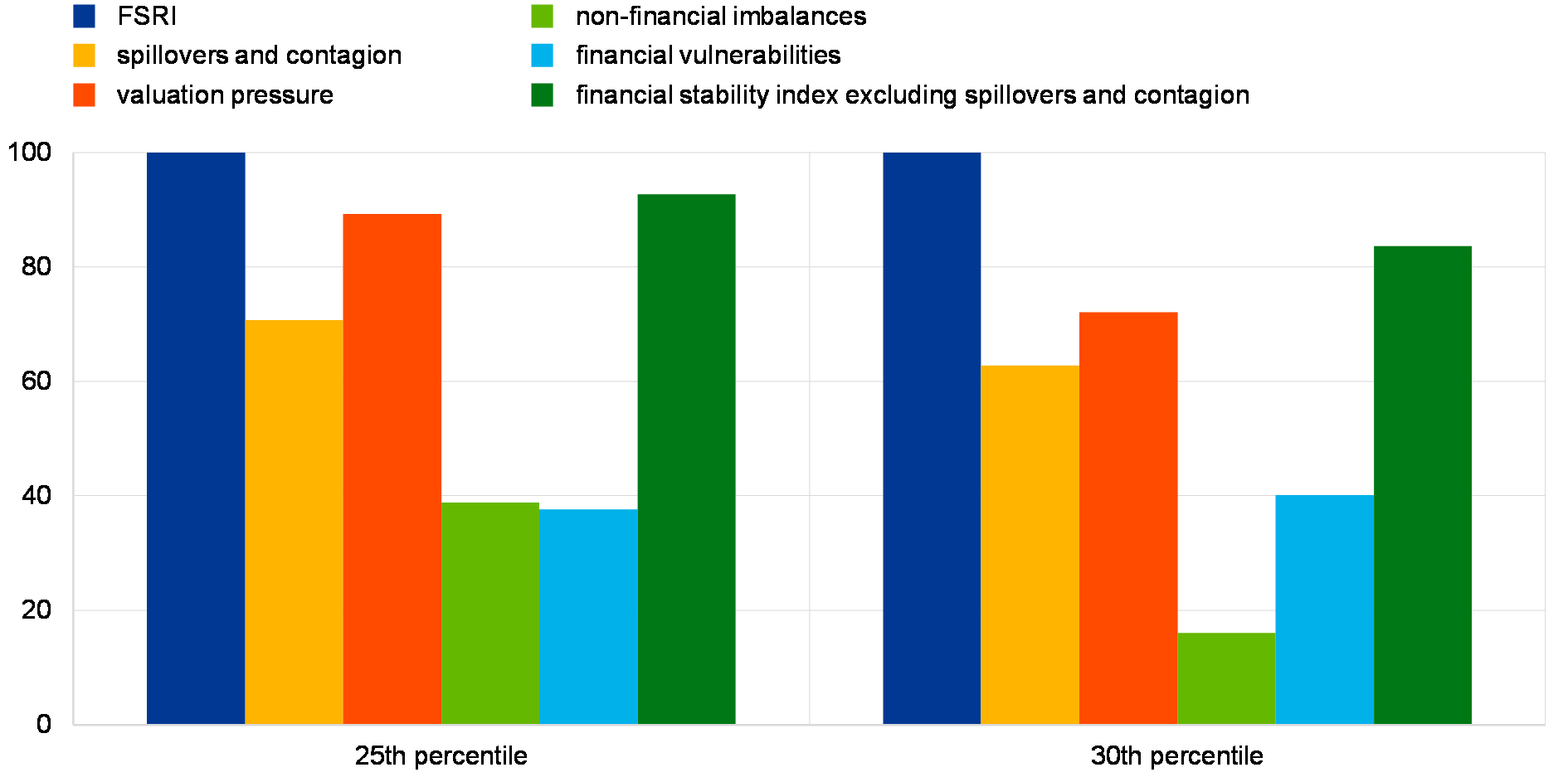
Source: ECB calculations.Notes: Out-of-sample forecast goodness-of-fit calculated relative to a historical quantile model. The forecasting performance of the FSRI is normalised to 100%. The sample period is from the first quarter of 2000 to the fourth quarter of 2017.
The forecasting power of the FSRI is strongest in the short term. Impulse response analysis suggests that GDP growth drops after an increase in the value of the indicator. The impact is significant, but phases out within one year. By design it is to be expected that the index will perform better for near-term predictions than over longer prediction horizons. The significant negative impulse responses within a year after the initial shock add evidence of the favourable near-term predictive properties of the index (see Chart A.5).
… while its forecasting power is concentrated in the short term
Impulse responses to a one standard deviation shock to the FSRI
(x-axis: quarters; y-axis: percentage points)
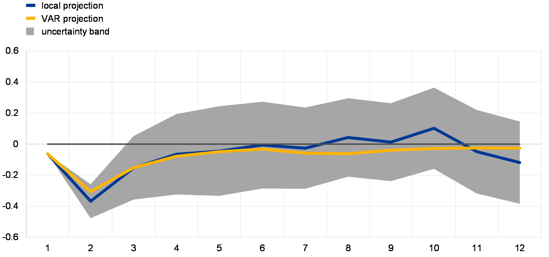
Source: ECB calculations.Notes: The impulse responses are measured as the response of quarterly GDP growth to a one standard deviation shock in the FSRI. The vector autoregression (VAR) is estimated with two lags and shocks are identified by Cholesky decomposition. The local projections are computed as in Jordà, Ò., “Estimation and Inference of Impulse Responses by Local Projections”, American Economic Review, No 95(1), 2005, pp. 161-182. The uncertainty band is computed from the local projections as +/- one standard deviation.
The most recent readings of the index point to a moderate increase in systemic risk owing to higher risk appetite and higher contagion and spillover risk. A low level of the indicator signals an overall contained level of systemic risk in the euro area in the short run, even if it has not declined to the levels observed before the financial crisis. The recent rise in the value of the FSRI is primarily driven by higher risk appetite and an increased contribution from spillover and contagion risks (see Chart A.6). While these two categories are still a drag on the overall level of the index from a historical perspective, their negative contributions declined in the second half of 2017. These categories were also the major contributors to systemic risks in the period 2007-2009 and during the sovereign debt crisis.
The level of the FSRI is strongly influenced by spillover and contagion and risk appetite indicators
Breakdown of the FSRI into its major components for selected periods
(index)

Sources: ECB and ECB calculations.
The overall dynamics of the index correspond to those of the composite indicator of systemic stress in financial markets (CISS), but there are distinct differences in the levels. The CISS dropped to historically low levels after the ECB’s Outright Monetary Transactions (OMT) announcement, which assuaged tensions in financial markets, while the FSRI receded more slowly (see Chart A.7).
The FSRI has exceeded the indicator of financial market stress in recent periods
FSRI and CISS
(7 Jan. 2000 to 11 May 2018; Q1 2000 to Q4 2017)

Sources: ECB and ECB calculations.Notes: The composite indicator of systemic stress in financial markets (CISS) is normalised to lie between 0 and 1. FSRI: quarterly frequency. CISS: weekly frequency, two-week moving average. At each point in time the index is standardised by its historical mean and standard deviation. The standardisation of the first 12 quarters is for that period.
4 Conclusions
This special feature proposes a new financial stability risk index (FSRI) that has near-term predictive power for deep recessions. Including the information content of spillover and contagion indicators seems to improve the performance of such a composite index in predicting economic tail events, i.e. episodes of financial turmoil that lead to deep recessions. The index presented here provides information on the impact that systemic risk could have on the real economy in the near term. A desirable extension would be to extend the prediction horizon. Such an application focusing on cyclical vulnerabilities is presented in Special Feature B.
- [1]See Adrian, T., Boyarchenko, N. and Giannone, D., “Vulnerable Growth”, Staff Reports, No 794 (revised), Federal Reserve Bank of New York, 2017.
- [2]See Giglio, S., Kelly, B. and Pruitt, S., “Systemic risk and the macroeconomy: An empirical evaluation”, Journal of Financial Economics, Vol. 119(3), 2016, pp. 457-471.
- [3]See also Constâncio, V., “Principles of Macroprudential Policy”, speech at the ECB-IMF Conference on Macroprudential Policy, Frankfurt am Main, 26 April 2016; and the special feature entitled “Systemic risk methodologies”, Financial Stability Review, ECB, June 2011.
- [4]See, for example, Schüler, Y.S., Hiebert, P.P. and Peltonen, T.A., “Characterising the financial cycle: a multivariate and time-varying approach”, Working Paper Series, No 1846, ECB, 2015.
- [5]However, the magnitude of cyclical imbalances will also have a bearing on the size of a potential economic downturn.
- [6]See Aikman, D., Kiley, M., Lee, S.J., Palumbo, M.G., Warusawitharana, M., “Mapping heat in the U.S. financial system”, Journal of Banking & Finance, Vol. 81, 2017, pp. 36-64.
- [7]See, for instance, Claessens, S., Kose, M.A. and Terrones, M.E., “What happens during recessions, crunches and busts?”, Economic Policy, No 24 (60), 2009, pp. 653-700; Alessi, L. and Detken, C., “‘Real time’ early warning indicators for costly asset price boom/bust cycles – a role for global liquidity”, Working Paper Series, No 1039, ECB, 2009; or Drehmann, M., Borio, C. and Tsatsaronis, K., “Anchoring Countercyclical Capital Buffers: The Role of Credit Aggregates”, International Journal of Central Banking, No 7(4), 2011, pp. 189-240.
- [8]Special Feature B also provides some evidence on the magnitude of crises.
- [9]The first three buckets are based on Aikman et al., op. cit.
- [10]See Benoit, S., Colliard, J.-E., Hurlin, C. and Pérignon, C., “Where the Risks Lie: A Survey on Systemic Risk”, Review of Finance, Vol. 21(1), 2017, pp. 109-152, who review 220 papers on systemic risk and identify four branches around which the literature can be classified: systemic risk measures, contagion, amplification mechanisms and systemic risk taking.
- [11]This relates to the finding that large drops in GDP can be attributed to the amplification mechanisms in the financial sector outlined in Adrian et al. (2017), op. cit.
- [12]Specifically, at each point in time the regression is estimated, where is the logarithm of real GDP and denotes the number of included lags. The GDP shocks are then computed as the residuals from this fitted regression.
- [13]The explanatory variables are standardised by removing the mean and dividing by the standard deviation.
- [14]Formally, the two stages can be expressed by the following equations: Stage 1(a): , 1(b): , where is a vector that contains the explanatory indicators from stage 1(a) and is the associated row-vector of estimated slope coefficients from that stage. Stage 2: , where is the estimated factor from the first stage. The time indexation of the coefficients is associated with the recursive out-of-sample methodology.
- [15]The index constitutes a consistent quantile forecast (see Giglio et al., op. cit.). In particular, the index provides a forecast of one-quarter-ahead shocks to GDP growth after scaling by its predictive sensitivity and adding a constant term. Both the predicative sensitivity and the constant term are recursively calculated with information up to time t.
- [16]The loss function is defined as , where is the quantile and is an indicator function that is equal to 1 when the condition x<0 is fulfilled and zero otherwise.
- [17]This approach is also used by Giglio et al., op. cit.
- [18]Koop, G. and Korobilis, D., “A new index of financial conditions”, European Economic Review, Vol. 71, 2014, pp. 101-116.


